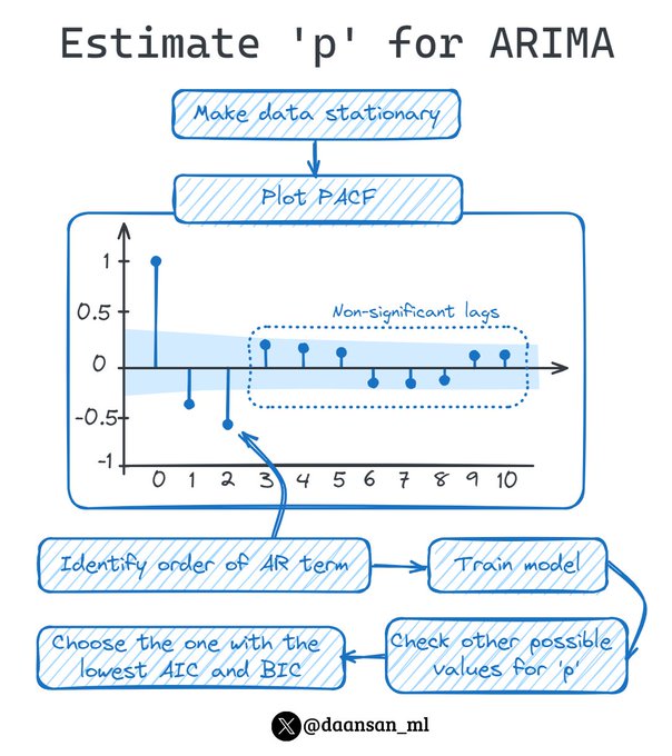
1️⃣ Ensure Stationarity: Start by ensuring the time series data is stationary. This is a crucial step as non-stationary data can lead to unreliable predictions. Differencing can be used to achieve stationarity.

2️⃣ ACF and PACF Plots: After ensuring stationarity, plot the Autocorrelation Function (ACF) and Partial Autocorrelation Function (PACF). A gradual decline in the ACF plot indicates a potential need for Autoregressive (AR) terms.

3️⃣ Identify Order of AR term: The order of the AR term (p) is chosen based on the PACF plot. Specifically, look for the lag value where partial autocorrelations become not significant. For example, if PACF cuts off at lag 2, set p=2.

4️⃣ Model Estimation and Fit: Fit the ARIMA model with the chosen p, and initial values for d (differencing) and q (moving average). This involves estimating the parameters of the model.

5️⃣ Model Diagnostics: Check the residuals of the model for any obvious patterns. Also, examine the ACF of residuals for significant autocorrelation, which could suggest that some information is not captured by the model.

6️⃣ Refinement: If necessary, adjust the value of p based on the diagnostic results. This is part of the iterative nature of building ARIMA models.

7️⃣ Cross-Validation / Information Criteria: Use information criteria like Akaike Information Criterion (AIC) or Bayesian Information Criterion (BIC) to compare models with different p values. Lower values indicate better fitting models.

Join more than 5k 💊MLPills subscribers and enjoy free Machine Learning and Data Science content straight to your email every week! 💊 Pill of the week: ML concept concisely explained 🤖 Tech Round-Up: hottest 5 AI news of the week 🎓 Learning materials

You should also join our newsletter, DSBoost🚀 Every week we share: 🔹Interviews 🔹Podcast notes 🔹Learning resources 🔹Interesting collections of content Subscribe for free👇👇

@daansan_ml Nicely explained!

@levikul09 Thanks Levi!

@daansan_ml 😊🙏Thank 🥺 mr Tsa

@LegaYcc Glad you liked it🙂🙂

@daansan_ml ACF and PACF both are important in identifying order of time series

@avikumart_ They're🙂

@daansan_ml Well explained, David.

@tinztwins Thanks!

@daansan_ml Learnt something new ;)

@_jaydeepkarale Glad to hear that🙂

@daansan_ml @rafaelbarbosa_s p = 2 ?

@leastsquared_ @rafaelbarbosa_s In this case yes! I've just realised that I forgot mentioning that🤦‍♂️